Impulse response equivalence

In this notebook we explore the equivalence between the two-layer model and a two-timescale impulse response approach.

Background

Following Geoffroy et al., 2013, Part 2, with notation altered to match our implementation, the two-layer model with efficacy (\(\epsilon\)) and state-dependent climate feedback can be written as

\begin{align} C \frac{dT}{dt} & = F - (\lambda_0 - a T) T - \epsilon \eta (T - T_D) \\ C_D \frac{dT_D}{dt} & = \eta (T - T_D) \end{align}

If the state-dependent feedback factor, \(a\), is non-zero, the two-layer model and impulse response approaches are not equivalent. However, if \(a=0\), they become the same.

Hereafter we assume \(a=0\), however this assumption should not be forgotten. In the case \(a=0\), the two-layer model can be written (adding an \(\epsilon\) for the deep-ocean equation too for simplicity later).

\begin{align} C \frac{dT}{dt} & = F - \lambda_0 T - \epsilon \eta (T - T_D) \\ \epsilon C_D \frac{dT_D}{dt} & = \epsilon \eta (T - T_D) \end{align}

In matrix notation we have

\begin{align} \frac{d\mathbf{X}}{dt} = \mathbf{A} \mathbf{X} + \mathbf{B} \end{align}

where \(\mathbf{X} = \begin{pmatrix}T \\T_D\end{pmatrix}\), \(\mathbf{A} = \begin{bmatrix} - \frac{\lambda_0 + \epsilon \eta}{C} & \frac{\epsilon \eta}{C} \\ \frac{\epsilon \eta}{\epsilon C_d} & -\frac{\epsilon \eta}{\epsilon C_d} \end{bmatrix}\) and \(\mathbf{B} = \begin{pmatrix} \frac{F}{C} \\ 0 \end{pmatrix}\).

As shown in Geoffroy et al., 2013, Part 1, \(\mathbf{A}\) can be diagonalised i.e. written in the form \(\mathbf{A} = \mathbf{\Phi} \mathbf{D} \mathbf{\Phi}^{-1}\), where \(\mathbf{D}\) is a diagonal matrix. Applying the solution given in Geoffroy et al., 2013, Part 1 to our impulse response notation, we have

\begin{align} \mathbf{D} = \begin{bmatrix} - \frac{1}{\tau_1} & 0 \\ 0 & - \frac{1}{\tau_2} \end{bmatrix} \end{align}

and

\begin{align} \mathbf{\Phi} = \begin{bmatrix} 1 & 1 \\ \phi_1 & \phi_2 \end{bmatrix} \end{align}

where

\begin{align} \tau_1 = \frac{C C_D}{2 \lambda_0 \eta} (b - \sqrt{\delta}) \end{align}

\begin{align} \tau_2 = \frac{C C_D}{2 \lambda_0 \eta} (b + \sqrt{\delta}) \end{align}

\begin{align} \phi_1 = \frac{C}{2 \epsilon \eta} (b^* - \sqrt{\delta}) \end{align}

\begin{align} \phi_2 = \frac{C}{2 \epsilon \eta} (b^* + \sqrt{\delta}) \end{align}

\begin{align} b = \frac{\lambda_0 + \epsilon \eta}{C} + \frac{\eta}{C_D} \end{align}

\begin{align} b^* = \frac{\lambda_0 + \epsilon \eta}{C} - \frac{\eta}{C_D} \end{align}

\begin{align} \delta = b^2 - 4 \frac{\lambda_0 \eta}{C C_D} \end{align}

Given this, we can re-write the system as

\begin{align} \frac{d\mathbf{X}}{dt} &= \mathbf{\Phi} \mathbf{D} \mathbf{\Phi}^{-1} \mathbf{X} + \mathbf{B} \\ \mathbf{\Phi}^{-1}\frac{d\mathbf{X}}{dt} &= \mathbf{D} \mathbf{\Phi}^{-1} \mathbf{X} + \mathbf{\Phi}^{-1} \mathbf{B} \\ \frac{d\mathbf{Y}}{dt} &= \mathbf{D} \mathbf{Y} + \mathbf{\Phi}^{-1} \mathbf{B} \\ \end{align}

Defining \(\mathbf{Y} = \begin{pmatrix} T_1 \\ T_2 \end{pmatrix}\), we have

\begin{align} \frac{d}{dt} \begin{pmatrix} T_1 \\ T_2 \end{pmatrix} = \begin{bmatrix} - \frac{1}{\tau_1} & 0 \\ 0 & - \frac{1}{\tau_2} \end{bmatrix} \begin{pmatrix} T_1 \\ T_2 \end{pmatrix} + \frac{1}{\phi_2 - \phi_1}\begin{bmatrix} \phi_2 & -1 \\ -\phi_1 & 1 \end{bmatrix} \begin{pmatrix} \frac{F}{C} \\ 0 \end{pmatrix} \end{align}

or,

\begin{align} \frac{dT_1}{dt} & = \frac{-T_1}{\tau_1} + \frac{\phi_2}{\phi_2 - \phi_1} \frac{F}{C} \\ \frac{dT_2}{dt} & = \frac{-T_2}{\tau_2} - \frac{\phi_1}{\phi_2 - \phi_1} \frac{F}{C} \end{align}

Re-writing, we have,

\begin{align} \frac{dT_1}{dt} & = \frac{1}{\tau_1} \left( \frac{\tau_1 \phi_2}{\phi_2 - \phi_1} \frac{F}{C} - T_1 \right) \\ \frac{dT_2}{dt} & = \frac{1}{\tau_2} \left( \frac{-\tau_2 \phi_1}{\phi_2 - \phi_1} \frac{F}{C} - T_2 \right) \end{align}

We can compare this to the notation of Millar et al., 2017 and see that

\begin{align} d_1 = \tau_1 \\ d_2 = \tau_2 \\ q_1 = \frac{\tau_1 \phi_2}{C(\phi_2 - \phi_1)} \\ q_2 = - \frac{\tau_2 \phi_1}{C(\phi_2 - \phi_1)} \\ \end{align}

Hence we have redemonstrated the equivalence of the two-layer model and a two-timescale impulse response model. Given the parameters of the two-layer model, we can now trivially derive the equivalent parameters of the two-timescale model. Doing the reverse is possible, but requires some more work in order to make a useable route drop out.

The first step is to follow Geoffroy et al., 2013, Part 1, and define two extra constants

\begin{align} a_1 = \frac{\phi_2 \tau_1}{C(\phi_2 - \phi_1)} \lambda_0 \\ a_2 = - \frac{\phi_1 \tau_2}{C(\phi_2 - \phi_1)} \lambda_0 \\ \end{align}

These constants have the useful property that \(a_1 + a_2 = 1\) (proof in Appendix A).

From above, we also see that

\begin{align} a_1 = \lambda_0 q_1 \\ a_2 = \lambda_0 q_2 \\ \end{align}

Hence

\begin{align} a_1 + a_2 = \lambda_0 q_1 + \lambda_0 q_2 = 1 \\ \lambda_0 = \frac{1}{q_1 + q_2} \end{align}

Next we calculate \(C\) via

\begin{align} \frac{q_1}{d_1} + \frac{q_2}{d_2} &= \frac{\phi_2}{C(\phi_2 - \phi_1)} - \frac{\phi_1}{C(\phi_2 - \phi_1)} = \frac{1}{C} \\ C &= \frac{d_1 d_2}{q_1 d_2 + q_2 d_1} \end{align}

We then use further relationships from Table 1 of Geoffroy et al., 2013, Part 1 (proof is left to the reader) to calculate the rest of the constants.

Firstly,

\begin{align} \tau_1 a_1 + \tau_2 a_2 = \frac{C + \epsilon C_D}{\lambda_0} \\ \epsilon C_D = \lambda_0 (\tau_1 a_1 + \tau_2 a_2) - C \end{align}

and then finally,

\begin{align} \tau_1 a_1 + \tau_2 a_2 = \frac{C + \epsilon C_D}{\lambda_0} \\ \epsilon \eta = \frac{\epsilon C_D}{\tau_1 a_2 + \tau_2 a_1} \end{align}

The final thing to notice here is that \(C_D\), \(\epsilon\) and \(\eta\) are not uniquely-defined. This makes sense, as shown by Geoffroy et al., 2013, Part 2, the introduction of the efficacy factor does not alter the behaviour of the system (it is still the same mathematical system) and so it is impossible for simply the two-timescale temperature response to uniquely define all three of these quantities. It can only define the products \(\epsilon C_D\) and \(\epsilon \eta\). Hence when translating from the two-timescale model to the two-layer model with efficacy, an explicit choice for the efficacy must be made. This does not alter the temperature response but it does alter the implied ocean heat uptake of the two-timescale model.

Long story short, when deriving two-layer model parameters from a two-timescale model, one must specify the efficacy.

Given that \(\mathbf{Y} = \mathbf{\Phi}^{-1} \mathbf{X}\) i.e. \(\mathbf{X} = \mathbf{\Phi} \mathbf{Y}\), we can also relate the impulse response boxes to the two layers.

\begin{aligned} \begin{pmatrix} T \\ T_D \end{pmatrix} = \begin{bmatrix} 1 & 1 \\ \phi_1 & \phi_2 \end{bmatrix} \begin{pmatrix} T_1 \\ T_2 \end{pmatrix} \\ \begin{pmatrix} T \\ T_D \end{pmatrix} = \begin{pmatrix} T_1 + T_2 \\ \phi_1 T_1 + \phi_2 T_2 \end{pmatrix} \end{aligned}

Finally, the equivalent of the two-timescale and two-layer models allows us to also calculate the heat uptake of a two-timescale impulse response model. It is given by

\begin{aligned} \text{Heat uptake} &= C \frac{dT}{dt} + C_D \frac{dT_D}{dt} \\ &= F - \lambda_0 T + (1 - \epsilon) \eta (T - T_D) \\ &= F - \lambda_0 (T_1 + T_2) + (1 - \epsilon) \eta ((1 - \phi_1) T_1 + (1 - \phi_2) T_2) \\ &= F - \lambda_0 (T_1 + T_2) - \eta (\epsilon - 1)((1 - \phi_1) T_1 + (1 - \phi_2) T_2) \end{aligned}

Running the code

Here we actually run the two implementations to explore their similarity.

import datetime as dt

import numpy as np
import pandas as pd
from openscm_units import unit_registry as ur
from scmdata.run import ScmRun, run_append

from openscm_twolayermodel import ImpulseResponseModel, TwoLayerModel

import matplotlib.pyplot as plt

/home/docs/checkouts/readthedocs.org/user_builds/openscm-two-layer-model/envs/stable/lib/python3.7/site-packages/openscm_twolayermodel/base.py:10: TqdmExperimentalWarning: Using `tqdm.autonotebook.tqdm` in notebook mode. Use `tqdm.tqdm` instead to force console mode (e.g. in jupyter console)
  import tqdm.autonotebook as tqdman

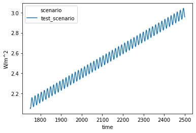
First we define a scenario to run.

time = np.arange(1750, 2501)
forcing = 0.05 * np.sin(time / 15 * 2 * np.pi) + 3.0 * time / time.max()

inp = ScmRun(
    data=forcing,
    index=time,
    columns={
        "scenario": "test_scenario",
        "model": "unspecified",
        "climate_model": "junk input",
        "variable": "Effective Radiative Forcing",
        "unit": "W/m^2",
        "region": "World",
    },
)
inp

<scmdata.ScmRun (timeseries: 1, timepoints: 751)>
Time:
        Start: 1750-01-01T00:00:00
        End: 2500-01-01T00:00:00
Meta:
          climate_model        model region       scenario   unit  \
        0    junk input  unspecified  World  test_scenario  W/m^2

                              variable
        0  Effective Radiative Forcing

# NBVAL_IGNORE_OUTPUT
inp.lineplot()

<AxesSubplot:xlabel='time', ylabel='W/m^2'>

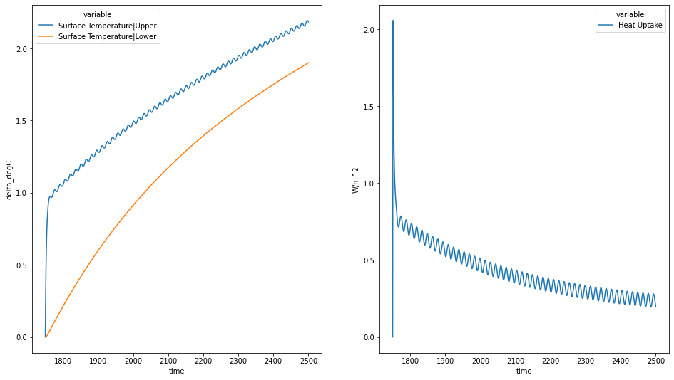
Next we run the two-layer model. In order for it to be convertible to a two-timescale model, we must turn state-dependence off (a=0).

two_layer_config = {
    "du": 55 * ur("m"),
    "efficacy": 1.2 * ur("dimensionless"),
    #     "efficacy": 1.0 * ur("dimensionless"),
    "a": 0 * ur("W/m^2/delta_degC^2"),
}

# NBVAL_IGNORE_OUTPUT
twolayer = TwoLayerModel(**two_layer_config)
res_twolayer = twolayer.run_scenarios(inp)
res_twolayer

<scmdata.ScmRun (timeseries: 4, timepoints: 751)>
Time:
        Start: 1750-01-01T00:00:00
        End: 2500-01-01T00:00:00
Meta:
           a (watt / delta_degree_Celsius ** 2 / meter ** 2) climate_model  \
        0                                                0.0     two_layer
        1                                                0.0     two_layer
        2                                                0.0     two_layer
        3                                                0.0     two_layer

           dl (meter)  du (meter)  efficacy (dimensionless)  \
        0        1200          55                       1.2
        1        1200          55                       1.2
        2        1200          55                       1.2
        3        1200          55                       1.2

           eta (watt / delta_degree_Celsius / meter ** 2)  \
        0                                             0.8
        1                                             0.8
        2                                             0.8
        3                                             0.8

           lambda0 (watt / delta_degree_Celsius / meter ** 2)        model region  \
        0                                           1.246667   unspecified  World
        1                                           1.246667   unspecified  World
        2                                           1.246667   unspecified  World
        3                                           1.246667   unspecified  World

           run_idx       scenario        unit                     variable
        0        0  test_scenario       W/m^2  Effective Radiative Forcing
        1        0  test_scenario  delta_degC    Surface Temperature|Upper
        2        0  test_scenario  delta_degC    Surface Temperature|Lower
        3        0  test_scenario       W/m^2                  Heat Uptake

# NBVAL_IGNORE_OUTPUT
fig = plt.figure(figsize=(16, 9))

ax = fig.add_subplot(121)
res_twolayer.filter(variable="*Temperature*").lineplot(hue="variable", ax=ax)

ax = fig.add_subplot(122)
res_twolayer.filter(variable="Heat Uptake").lineplot(hue="variable", ax=ax)

<AxesSubplot:xlabel='time', ylabel='W/m^2'>

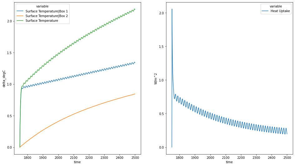
Next we get the parameters with which we get the equivalent impulse response model.

two_timescale_paras = twolayer.get_impulse_response_parameters()
two_timescale_paras

{'d1': 103454323.57029569 <Unit('joule / watt')>,
 'd2': 11181891933.114195 <Unit('joule / watt')>,
 'q1': 0.4465999986742509 <Unit('delta_degree_Celsius * meter ** 2 / watt')>,
 'q2': 0.3555390387589074 <Unit('delta_degree_Celsius * meter ** 2 / watt')>,
 'efficacy': 1.2 <Unit('dimensionless')>}

# NBVAL_IGNORE_OUTPUT
impulse_response = ImpulseResponseModel(**two_timescale_paras)
res_impulse_response = impulse_response.run_scenarios(inp)
res_impulse_response

<scmdata.ScmRun (timeseries: 5, timepoints: 751)>
Time:
        Start: 1750-01-01T00:00:00
        End: 2500-01-01T00:00:00
Meta:
                            climate_model  d1 (joule / watt)  d2 (joule / watt)  \
        0  two_timescale_impulse_response       1.034543e+08       1.118189e+10
        1  two_timescale_impulse_response       1.034543e+08       1.118189e+10
        2  two_timescale_impulse_response       1.034543e+08       1.118189e+10
        3  two_timescale_impulse_response       1.034543e+08       1.118189e+10
        4  two_timescale_impulse_response       1.034543e+08       1.118189e+10

           efficacy (dimensionless)        model  \
        0                       1.2  unspecified
        1                       1.2  unspecified
        2                       1.2  unspecified
        3                       1.2  unspecified
        4                       1.2  unspecified

           q1 (delta_degree_Celsius * meter ** 2 / watt)  \
        0                                         0.4466
        1                                         0.4466
        2                                         0.4466
        3                                         0.4466
        4                                         0.4466

           q2 (delta_degree_Celsius * meter ** 2 / watt) region  run_idx  \
        0                                       0.355539  World        0
        1                                       0.355539  World        0
        2                                       0.355539  World        0
        3                                       0.355539  World        0
        4                                       0.355539  World        0

                scenario        unit                     variable
        0  test_scenario       W/m^2  Effective Radiative Forcing
        1  test_scenario  delta_degC    Surface Temperature|Box 1
        2  test_scenario  delta_degC    Surface Temperature|Box 2
        3  test_scenario  delta_degC          Surface Temperature
        4  test_scenario       W/m^2                  Heat Uptake

# NBVAL_IGNORE_OUTPUT
fig = plt.figure(figsize=(16, 9))

ax = fig.add_subplot(121)
res_impulse_response.filter(variable="*Temperature*").lineplot(
    hue="variable", ax=ax
)

ax = fig.add_subplot(122)
res_impulse_response.filter(variable="Heat Uptake").lineplot(
    hue="variable", ax=ax
)

<AxesSubplot:xlabel='time', ylabel='W/m^2'>

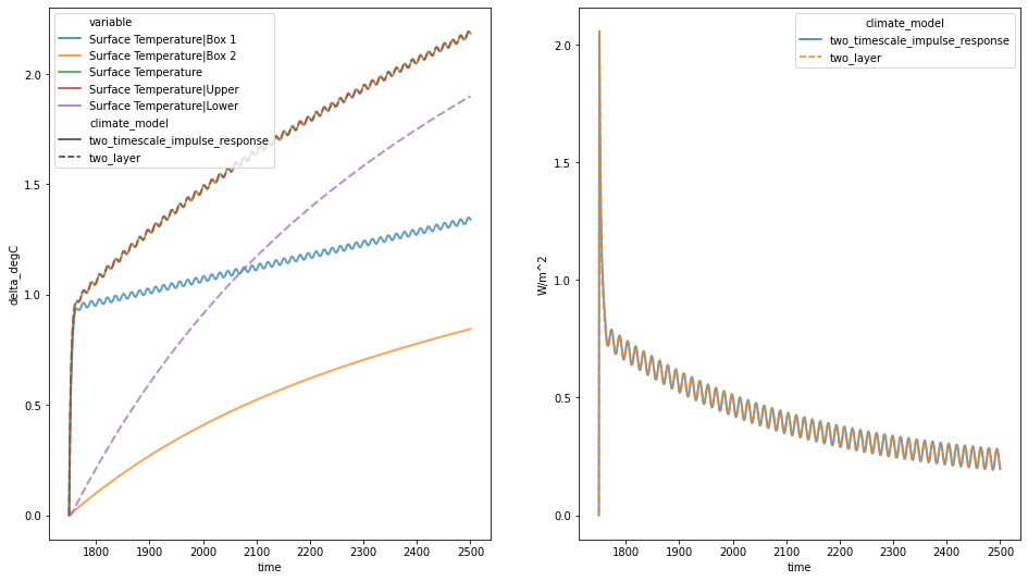
We can compare the two responses as well.

# NBVAL_IGNORE_OUTPUT
combined = run_append([res_impulse_response, res_twolayer])
combined

<scmdata.ScmRun (timeseries: 9, timepoints: 751)>
Time:
        Start: 1750-01-01T00:00:00
        End: 2500-01-01T00:00:00
Meta:
           a (watt / delta_degree_Celsius ** 2 / meter ** 2)  \
        0                                                NaN
        1                                                NaN
        2                                                NaN
        3                                                NaN
        4                                                NaN
        5                                                0.0
        6                                                0.0
        7                                                0.0
        8                                                0.0

                            climate_model  d1 (joule / watt)  d2 (joule / watt)  \
        0  two_timescale_impulse_response       1.034543e+08       1.118189e+10
        1  two_timescale_impulse_response       1.034543e+08       1.118189e+10
        2  two_timescale_impulse_response       1.034543e+08       1.118189e+10
        3  two_timescale_impulse_response       1.034543e+08       1.118189e+10
        4  two_timescale_impulse_response       1.034543e+08       1.118189e+10
        5                       two_layer                NaN                NaN
        6                       two_layer                NaN                NaN
        7                       two_layer                NaN                NaN
        8                       two_layer                NaN                NaN

           dl (meter)  du (meter)  efficacy (dimensionless)  \
        0         NaN         NaN                       1.2
        1         NaN         NaN                       1.2
        2         NaN         NaN                       1.2
        3         NaN         NaN                       1.2
        4         NaN         NaN                       1.2
        5      1200.0        55.0                       1.2
        6      1200.0        55.0                       1.2
        7      1200.0        55.0                       1.2
        8      1200.0        55.0                       1.2

           eta (watt / delta_degree_Celsius / meter ** 2)  \
        0                                             NaN
        1                                             NaN
        2                                             NaN
        3                                             NaN
        4                                             NaN
        5                                             0.8
        6                                             0.8
        7                                             0.8
        8                                             0.8

           lambda0 (watt / delta_degree_Celsius / meter ** 2)        model  \
        0                                                NaN   unspecified
        1                                                NaN   unspecified
        2                                                NaN   unspecified
        3                                                NaN   unspecified
        4                                                NaN   unspecified
        5                                           1.246667   unspecified
        6                                           1.246667   unspecified
        7                                           1.246667   unspecified
        8                                           1.246667   unspecified

           q1 (delta_degree_Celsius * meter ** 2 / watt)  \
        0                                         0.4466
        1                                         0.4466
        2                                         0.4466
        3                                         0.4466
        4                                         0.4466
        5                                            NaN
        6                                            NaN
        7                                            NaN
        8                                            NaN

           q2 (delta_degree_Celsius * meter ** 2 / watt) region  run_idx  \
        0                                       0.355539  World        0
        1                                       0.355539  World        0
        2                                       0.355539  World        0
        3                                       0.355539  World        0
        4                                       0.355539  World        0
        5                                            NaN  World        0
        6                                            NaN  World        0
        7                                            NaN  World        0
        8                                            NaN  World        0

                scenario        unit                     variable
        0  test_scenario       W/m^2  Effective Radiative Forcing
        1  test_scenario  delta_degC    Surface Temperature|Box 1
        2  test_scenario  delta_degC    Surface Temperature|Box 2
        3  test_scenario  delta_degC          Surface Temperature
        4  test_scenario       W/m^2                  Heat Uptake
        5  test_scenario       W/m^2  Effective Radiative Forcing
        6  test_scenario  delta_degC    Surface Temperature|Upper
        7  test_scenario  delta_degC    Surface Temperature|Lower
        8  test_scenario       W/m^2                  Heat Uptake

To within numerical errors they are equal.

# NBVAL_IGNORE_OUTPUT
fig = plt.figure(figsize=(16, 9))

ax = fig.add_subplot(121)
combined.filter(variable="*Temperature*").lineplot(
    hue="variable", style="climate_model", alpha=0.7, linewidth=2, ax=ax
)
ax.legend(loc="upper left")

ax = fig.add_subplot(122)
combined.filter(variable="Heat Uptake").lineplot(
    hue="climate_model", style="climate_model", alpha=0.7, linewidth=2, ax=ax
)

<AxesSubplot:xlabel='time', ylabel='W/m^2'>

Appendix A

We begin with the definitions of the \(a\) constants,

\begin{align} a_1 = \frac{\phi_2 \tau_1}{C(\phi_2 - \phi_1)} \lambda_0 \\ a_2 = - \frac{\phi_1 \tau_2}{C(\phi_2 - \phi_1)} \lambda_0 \\ \end{align}

We then have

\begin{align} a_1 + a_2 &= \frac{\phi_2 \tau_1}{C(\phi_2 - \phi_1)} \lambda_0 - \frac{\phi_1 \tau_2}{C(\phi_2 - \phi_1)} \lambda_0 \\ &= \frac{\lambda_0}{C(\phi_2 - \phi_1)} (\phi_2 \tau_1 - \phi_1 \tau_2) \end{align}

Recalling the definition of the \(\phi\) parameters,

\begin{align} \phi_1 = \frac{C}{2 \epsilon \eta} (b^* - \sqrt{\delta}) \end{align}

\begin{align} \phi_2 = \frac{C}{2 \epsilon \eta} (b^* + \sqrt{\delta}) \end{align}

We have,

\begin{align} \phi_2 - \phi_1 = \frac{C \sqrt{\delta}}{\epsilon \eta} \end{align}

Recalling the definition of the \(\tau\) parameters,

\begin{align} \tau_1 = \frac{C C_D}{2 \lambda_0 \eta} (b - \sqrt{\delta}) \end{align}

\begin{align} \tau_2 = \frac{C C_D}{2 \lambda_0 \eta} (b + \sqrt{\delta}) \end{align}

We have,

\begin{align} \phi_2 \tau_1 - \phi_1 \tau_2 &= \frac{C}{2 \epsilon \eta} (b^* + \sqrt{\delta}) \times \frac{C C_D}{2 \lambda_0 \eta} (b - \sqrt{\delta}) - \frac{C}{2 \epsilon \eta} (b^* - \sqrt{\delta}) \times \frac{C C_D}{2 \lambda_0 \eta} (b + \sqrt{\delta}) \\ &= \frac{C^2 C_d}{4 \epsilon \eta^2 \lambda_0} \left[ (b^* + \sqrt{\delta}) (b - \sqrt{\delta}) - (b^* - \sqrt{\delta}) (b + \sqrt{\delta}) \right] \\ &= \frac{C^2 C_d}{4 \epsilon \eta^2 \lambda_0} \left[ b^*b + b\sqrt{\delta} -b^*\sqrt{\delta} - \delta - bb^* + b\sqrt{\delta} - b^*\sqrt{\delta} + \delta \right] \\ &= \frac{C^2 C_d}{2 \epsilon \eta^2 \lambda_0} \left[ b\sqrt{\delta} -b^*\sqrt{\delta} \right] \\ &= \frac{C^2 C_d \sqrt{\delta}}{2 \epsilon \eta^2 \lambda_0} \left[ b -b^*\right] \end{align}

Recalling the definition of the \(b\) parameters,

\begin{align} b = \frac{\lambda_0 + \epsilon \eta}{C} + \frac{\eta}{C_D} \end{align}

\begin{align} b^* = \frac{\lambda_0 + \epsilon \eta}{C} - \frac{\eta}{C_D} \end{align}

We then have

\begin{align} \phi_2 \tau_1 - \phi_1 \tau_2 &= \frac{C^2 C_d \sqrt{\delta}}{2 \epsilon \eta^2 \lambda_0} \left[ \frac{2\eta}{C_D} \right] \\ &= \frac{C^2 \sqrt{\delta}}{\epsilon \eta \lambda_0} \end{align}

Putting it all back together,

\begin{align} a_1 + a_2 &= \frac{\lambda_0}{C(\phi_2 - \phi_1)} (\phi_2 \tau_1 - \phi_1 \tau_2) \\ &= \frac{\lambda_0}{C} \frac{\epsilon \eta}{C \sqrt{\delta}} \frac{C^2 \sqrt{\delta}}{\epsilon \eta \lambda_0} \\ &= 1 \end{align}